Visualizing the Heart of Some PRNGs
A major point I made in the PCG paper was that we get useful insights by testing small versions of PRNGs. These mini versions may be too small to be useful in practice, but their structure will give us a good sense about the structure of their larger counterparts.
In this post, we'll look at 16-bit versions of several popular PRNGs, and draw some “randomgrams” to get a sense of their structure. In particular, we're going to look at the pattern of occurrences of pairs in the output, in other words which pairs of outputs occur once, which never occur at all, and which occur multiple times.
Randograms & The Expected Histogram
For much of this post, we'll be looking at “randograms”, which are 2D plots of the state space of a tiny 16-bit version of a generation technique with 8-bit output. Randograms help drive our intuitions. We can expect that phenomena we see at the small scale will continue at larger scales (where the equivalent visualizations would be so huge as to be unmanageable). As a first approximation, if a randogram looks “kinda random”, it doesn't prove that we have sufficient statistical quality, but, on the other hand, if something leaps out to our eye as clearly having obvious structure, we know that we are looking at a flaw.
The randograms we'll use in this post are a little different from the ones in the PCG paper. Here the intensity of each dot represents how many occurrences there are of the pair indicated by the (x,y) coordinate of the pixel. Every occurrence halves the intensity of the pixel. With zero occurrences it is white (100%), with one it is 50% grey, with two 25% grey, etc.
We'll also give a histogram of the data. For a random sample of 65,536 points, we would expect the following (binomial) distribution for pair occurrences:
Occur   Count
  0     24109.163
  1     24109.531
  2     12054.765
  3     4018.1939
  4     1004.5178
  5     200.89436
  6     33.480350
  7     4.7825422
  8     0.5977631
  9     0.0664110
 10     0.0066403
LCG Family & PCG
We'll begin by looking at a 16-bit LCG with 8-bit output, and see the difference that one of the standard PCG output functions makes.
Linear Congruential Generator
We'll use a 16-bit LCG with a multiplier of 25385, since that's what
PCG uses for 16-bit-state LCGs. If we used a different multiplier,
the patterns below would be different but the general idea would be
the same.
The High Eight Bits
Sometimes I've been known to say, “LCGs are too smooth”, and we can see that there is a clear repetitive structure. Also, most of the points where there are two of the same pair (the small number of darker dots), are right next to light dots from a pair being omitted.

The histogram of occurrences is wrong. Too many pairs occur exactly once. Again, we can see this as a “too smooth” issue.
Histogram for lcg25385high:
Occur   Count
  0     7936
  1     49664
  2     7936
The Low Eight Bits
The low bits of a power-of-two LCG are terrible. They have a short period, so we shouldn't expect much good here.
And the histogram is, unsurprisingly, also terrible.
Histogram for lcg25385low:
Occur   Count
  0     65280
  1     0
  2     0
  3     0
  4     0
  5     0
  :     :
  255   0
  256   256
PCG 8 (XSH RR)
The tiny pcg8 quarter-sized cousin of pcg32 uses the above LCG, but
puts the state through the XSH RR output function. Here's the result:

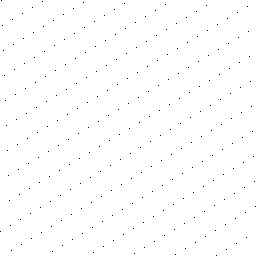
It looks right! Random, not regular. We'll see more of these for other generators, but this is what a “random looking” randogram should look like.
Likewise, the histogram is good. It's consistent with a random sample.
Histogram for pcg8:
Occur   Count
  0     24069
  1     24045
  2     12251
  3     3971
  4     971
  5     192
  6     30
  7     4
  8     3
One concern you might have is that although the above histogram is consistent with a random sample, we seem to be “baking in” the characteristics of one particular histogram, which we will now be stuck with forever, and that might feel like a kind of bias; some pairs are more likely than others! I agree! That's why PCG has streams, which come from varying the LCG additive constant.
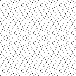
Here are the results for four randomly chosen additive constants,
.png)
.png)
.png)
.png)
and their histograms,
Histogram for pcg8(0,0x7564):
Occur   Count
  0 24150
  1 24018
  2 12085
  3 4062
  4 984
  5 203
  6 27
  7 7

Histogram for pcg8(0,0x03ff):
Occur   Count
  0 24120
  1 23901
  2 12401
  3 3919
  4 950
  5 202
  6 36
  7 6
  8 1

Histogram for pcg8(0,0x1bd1):
Occur   Count
  0 24249
  1 23792
  2 12299
  3 3945
  4 996
  5 214
  6 32
  7 7
  8 2

Histogram for pcg8(0,0x27ca):
Occur   Count
  0 24129
  1 23963
  2 12222
  3 4042
  4 946
  5 195
  6 31
  7 6
  8 2
The histograms are different for each stream, and we have 215 streams to choose from. Thus we aren't locked into always having the same histogram.
If you stare at the four randograms above long enough, you may be able to convince yourself that perhaps we're just “kinda scrolling around” on the same random picture. But if we really were just scrolling the same picture, the histograms would be the same, so that's not quite the case. Nevertheless, these streams aren't different enough for me to feel like they are statistically independent. But they are usefully distinct.
If you find the whole question of streams interesting, see my post on streams in PCG for more about this area. The short version is that the steams would be more different if we varied the PCG permutation or the LCG multiplier.
Marsaglia's XorShift Family
Okay, now let's move on to looking at classic XorShift generators as proposed by Marsaglia. Whereas with LCGs you can vary the increment parameter to get different streams, for XorShift, varying the algorithmic parameters to get different streams is a trickier affair—improper parameters will result in a generator that is not full period and, as Vigna discovered, some parameters that conform to the mathematical rules suggested by Marsaglia aren't very good when tested. For my implementation of XorShift, I hand selected just four shift parameter combinations to make four different generators, calling the variants A, B, C, and D.
(For the first part of our discussion, you may start to question my choices, but things will get better, I assure you.)
Vanilla XorShift
Low Bits, Parameterizations A, B, C, & D


Histogram for xorshift16low8a:
Occur   Count
  0     32768
  1     1
  2     32767

Histogram for xorshift16low8b:
Occur   Count
  0     57344
  1     0
  2     0
  3     0
  4     0
  5     0
  6     0
  7     1
  8     8191

Histogram for xorshift16low8c:
Occur   Count
  0     61440
  1     0
  2     0
  3     0
  4     0
  5     0
  :     :
  14    0
  15    1
  16    4095

Histogram for xorshift16low8d:
Occur   Count
  0     32768
  1     1
  2     32767
Well, these are certainly quite different from each other! I sometimes say “(G)LFSRs are too lumpy”, and you may be able to see from both the diagrams and the histograms reasons to agree (although my vague intuitive “lumpiness” characterization applies in other ways, too, including the way that most LFSRs get mired in areas of neighboring bad states).
High Bits, Parameterizations A, B, C, & D


Histogram for xorshift16high8a:
Occur   Count
  0     32768
  1     1
  2     32767

Histogram for xorshift16high8b:
Occur   Count
  0     32768
  1     1
  2     32767

Histogram for xorshift16high8c:
Occur   Count
  0     57344
  1     0
  2     0
  3     0
  4     0
  5     0
  6     0
  7     1
  8     8191

Histogram for xorshift16high8d:
Occur   Count
  0     32768
  1     1
  2     32767
Funky! I think you can see why you want to add a decent output function to condition the output into something more reasonable.
XorShift with Untruncated (Half-State) Multiply
If you look on-line, you'll see people producing generators that just apply an MCG multiplication to what would otherwise be the output of the XorShift generator.
Unfortunately, that's not really the right thing to do, as we can see. The randograms will be different, but not really better.
Low Bits, Parameterizations A, B, C, & D


When we look at the histograms, we see that nothing has really changed; we've shuffled the values around, but not made any difference.
Histogram for xorshift16lowstar8a:
Occur   Count
  0     32768
  1     1
  2     32767

Histogram for xorshift16lowstar8b:
Occur   Count
  0     57344
  1     0
  2     0
  3     0
  4     0
  5     0
  6     0
  7     1
  8     8191

Histogram for xorshift16lowstar8c:
Occur   Count
  0     61440
  1     0
  2     0
  3     0
  4     0
  5     0
  :     :
  14    0
  15    1
  16    4095

Histogram for xorshift16lowstar8d:
Occur   Count
  0     32768
  1     1
  2     32767
High Bits, Parameterizations A, B, C, & D
The same applies to the high bits.


Histogram for xorshift16highstar8a:
Occur   Count
  0     32768
  1     1
  2     32767

Histogram for xorshift16highstar8b:
Occur   Count
  0     32768
  1     1
  2     32767

Histogram for xorshift16highstar8c:
Occur   Count
  0     57344
  1     0
  2     0
  3     0
  4     0
  5     0
  6     0
  7     1
  8     8191

Histogram for xorshift16highstar8d:
Occur   Count
  0     32768
  1     1
  2     32767
XorShift with Truncated (Full-State) Multiply
Let's try a different output function: take all 16 bits of XorShift state, perform a 16-bit MCG multiply, and then truncate the result, keeping the high eight bits. Suddenly, our four previously horrible looking generators are all looking quite wonderful!


And the histograms look right too!
Histogram for xorshift16star8a:
Occur   Count
  0     23444
  1     24815
  2     12358
  3     3863
  4     886
  5     151
  6     17
  7     2

Histogram for xorshift16star8b:
Occur   Count
  0     23979
  1     24209
  2     12191
  3     3943
  4     1005
  5     166
  6     38
  7     3
  8     2

Histogram for xorshift16star8c:
Occur   Count
  0     23969
  1     24290
  2     12101
  3     3927
  4     1029
  5     179
  6     36
  7     5

Histogram for xorshift16star8d:
Occur   Count
  0     23483
  1     24791
  2     12277
  3     3932
  4     898
  5     131
  6     22
  7     1
  8     1
All the above are plausible. (I like it when things work the way they
should!) Of course, we only have four different histograms, unlike the
215 we had with 16-bit pcg8. There are ways to add more
streams, but a small number of streams is the best we can get “for
free” via reparameterization.
Xoroshiro Family
So, what about Vigna's Xoroshiro family? He doesn't provide tiny versions, but the theory he's using is just Marsaglia's, so it isn't very hard to make versions at other sizes.
Vanilla Xoroshiro (Raw Output)


Histogram for xoroshiro16rawS0:
Occur   Count
  0     1
  1     65535

Histogram for xoroshiro16rawS1:
Occur   Count
  0     1
  1     65535
Other than a missing (0,0) pair (top corner of the square), we can
see that the two halves of Xoroshiro state are equidistributed. We
don't have a random sample here, we have two-dimensional
equidistribution, with a single occurrence of each pair. That
arrangement has a certain elegance to it, but from a statistical
standpoint, it's still flawed. Yes, there are no pairs omitted
(except for the missing (0,0) pair), but there are also no
repeats. Statistically, repeats should happen.
But that's the internal state of Xoroshiro, not the output.
Xoroshiro with Additive Output Function
Vigna's output function is to add together the two halves of the state. Here's the end product:
Histogram for xoroshiro16plus8:
Occur   Count
  0     35273
  1     12781
  2     7773
  3     4845
  4     2707
  5     1449
  6     402
  7     277
  8     13
  9     15
  10    1
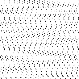
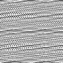
From the graph and the histogram, we can see that these results aren't good! Not as bad, perhaps as an LCG or vanilla XorShift, but nevertheless much worse that Truncated XorShift*, PCG, or numerous other generators.
You might wonder if these issues really do persist in the larger sizes of Xoroshiro, like Xoroshiro128+. Yes, they do. The detection techniques are different from drawing a picture (after all, we can't plot out the whole period of a 128-bit generator), but once we know what we're looking for, it isn't too hard to find with some hand-coded exploration. Given the length of this post, I'll leave that part as an exercise for the reader! But it is a tall order to expect a general PRNG test suite to find these kinds of issues in a 128-bit generator with 64-bit output, since we're talking about tracking repeats of pairs of 64-bit values. As I outlined in my previous post, 128-bits is well into “too big to fail” territory, where the amount of data needed to discover the flaw is just too vast.
Xoroshiro with Truncated (Full-State) Multiply
If we swap out Vigna's output function for an old-school truncated multiply, we get much better results.

Histogram for xoroshiro16star8:
Occur   Count
  0     23964
  1     24135
  2     12303
  3     3980
  4     951
  5     171
  6     29
  7     3
Much better! But not what Vigna did though. Not what you get if you're using Xoroshiro128+.
Conclusion
Looking at cut-down versions of PRNGs tells you useful things. I also think they show the value of a certain kind of playfulness and informality. It's valuable to be able to express yourself in mathematical formalisms, but writing a program that just shows you what things look like can sometimes give you more insight than a proof, especially in the world of random number generation where mathematics alone currently fails to characterize all that is going on.